Numerical integration via the midpoint rule and the trapezoid rule
This is a supplementary post to a series of posts I’m writing about the CPBRT renderer, an implementation of Pharr, Jakob and Humphrey’s PBRT.
Numerical integration is used to evaluate definite integrals of functions whose antiderivatives can’t be found analytically because either the integrand is not in closed form or the interval or domain of integration is not continuous. The integral equation that describes light scattering, \[L_{o}(p,\omega_{o}) = \int_{\Omega=H^2(n)} f_{r}(p,\omega_{o},\omega_{i})L_{i}(p,\omega_{i})\vert\cos \theta_{i}\vert \, d\omega_{i}\]
is a good case in point, because the set \(\Omega\) of directions usually isn’t the full hemisphere or sphere, but one that is “patchy” due to occlusion of subsets of directions.
Numerical methods produce approximations of the value of an integral, not the exact one. Given the exact value \(x\) and the computed approximation \(c\) produced by a numerical method, the error can be measured in 2 ways: \[error_{absolute} = \vert c-x \vert\]
and \[error_{relative} = \frac{\vert c-x \vert}{\vert x \vert},\quad if\,x\neq0\]
One can then imagine a procedure that aims at minimizing the approximation error measured with respect to a reference.
For the 2 approximation methods that I’ll describe next, the absolute error has a known upper bound; I’ll come back to this point at the end of the post. These 2 methods, the midpoint rule and the trapezoid rule, aren’t exactly what PBRT (or CPBRT for that matter) uses for evaluating integrals, but I believe that studying them to some extent serves as a warmup exercise before delving Monte Carlo integration.
Midpoint rule approximation
Suppose that \(f\) is defined and integrable on \([a, b]\). The midpoint rule approximation to \(\int_{a}^{b}f(x) \, dx\) using \(n\) regularly spaced subintervals of \([a, b]\) is \[\begin{aligned} M(n) &= f(m_{1})\Delta x + f(m_{2}) \Delta x +...+ f(m_{n}) \Delta x \\ &= \sum_{k=1}^{n}f(\frac{x_{k-1}+x_{k}}{2}) \Delta x \end{aligned}\]
where \(\Delta x = \frac{b-a}{n}\), \(x_{0}=a\), \(x_{k}=a+k\Delta x\), and \(m_{k}=\frac{x_{k-1}+x_{k}}{2}\) is the midpoint of \([x_{k-1}, x_{k}]\), for \(k=1,2,...,n\).
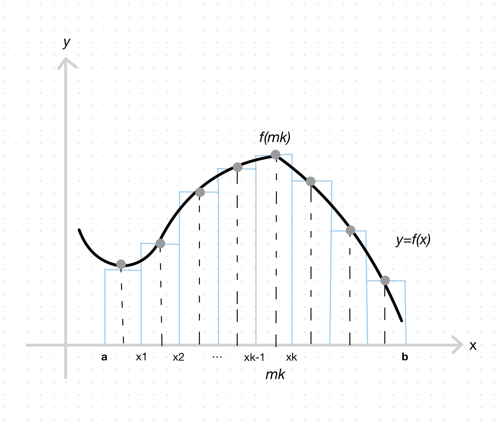
In this definition one can recognize the midpoint Riemann sum that approximates the area under the curve by adding up the areas of contiguous rectangles. The definite integral is thus computed from regularly spaced samples of the domain of integration and the corresponding value of the integrand.
Trapezoid rule approximation
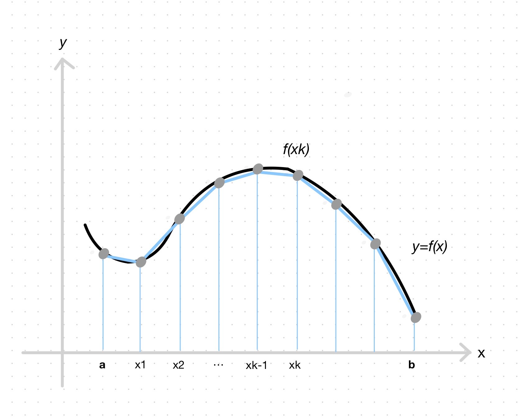
Suppose that \(f\) is defined and integrable on \([a, b]\). The trapezoid rule approximation to \(\int_{a}^{b}f(x) \, dx\) using \(n\) regularly spaced subintervals of \([a, b]\) is \[\begin{aligned} T(n) &= \frac{f(x_{0})+f(x_{1})}{2}\Delta x + \frac{f(x_{1})+f(x_{2})}{2}\Delta x + ... + \frac{f(x_{n-1})+f(x_{n})}{2}\Delta x \\ &= \Big(\frac{1}{2}f(x_{0})+\sum_{k=1}^{n-1}f(x_{k})+\frac{1}{2}f(x_{n})\Big) \Delta x \end{aligned}\]
where \(\Delta x = \frac{b-a}{n}\) and \(x_{k}=a+k\Delta x\), for \(k=0,1,...,n\).
Observe that the trapezoid rule approximation is like the midpoint rule approximation, but it adds up the areas of trapezoids instead of rectangles, where the net area of the \(k\)th trapezoid is given by \[\frac{f(x_{k-1})+f(x_{x})}{2}\Delta x\]
Measuring the approximation error
As mentioned in the introduction, the upper bounds of the absolute errors of the midpoint rule approximation and the trapezoid approximation are known and can be computed.
Suppose that \(f''\) is continuous on the interval \([a, b]\) and that \(k\) is a real number such that \(\vert f''(x) \leq k\vert\), for all \(x\) in \([a, b]\). The absolute error of the midpoint rule approximation to \(\int_{a}^{b}f(x) \, dx\) with \(n\) subintervals has the following upper bound \[error_{M} \leq \frac{k(b-a)}{24}(\Delta x)^2\]
and similarly for the trapezoid rule approximation with \(n\) subintervals \[error_{T} \leq \frac{k(b-a)}{12}(\Delta x)^2\]
where \(\Delta x = \frac{b-a}{n}\).
By computing these bounds and establishing an acceptable error magnitude, you may increase \(n\) (thereby increasing the amount of computation) until the corresponding upper bound is acceptable, all without actually knowing the true value of the integral or the error. (Note, however, that you must be able to obtain the 2nd derivative of the integrand.).
Closing remarks
One of the many reasons these 2 methods aren’t used by PBRT is that as the number of samples of the function increases (the number of subintervals in our exposition above), the rate at which the approximation convergences to the true value of the integral is very poor for the higher-dimensional and discontinuous integrals that are common in rendering. Monte Carlo integration, on the other hand, is very effective at estimating the value of just such integrals; I hope to cover that method in a future post.
I refer the interested reader to Calculus, by Tom M. Apostol, 1991, for more on these numerical integration methods.