Sampling and reconstruction in CPBRT
Sampling is the process of taking discrete values of a continuous function. Reconstruction is the process of converting the discrete samples back to a continuous function, which tries to approximate the original one as much as possible. In rendering, the scene’s incident radiance is the continuous function defined over the film plane that we try to approximate by sampling the incident radiance value of discrete pixels. Sampling is done by tracing rays and the result is a digital pixel image; we can say that the image is a discretization of the incident radiance function. Reconstruction is then performed by the display, typically via some form of interpolation, and the resulting function is defined over the surface of the display.
That’s sampling and reconstruction in a nutshell. The goal of this post is to introduce some of the sampling and reconstruction theory behind (C)PBRT to elaborate on that description. In particular, we’ll explore some of the main ideas of Fourier analysis (and why it is relevant), the ideal way of doing sampling and reconstruction, the problems that arise and ways to mitigate them, and the sampling algorithms and filters that are currently implemented in CPBRT.
The Dirac delta distribution
The Dirac delta distribution \(\delta(x)\) is one that satisfies \[\begin{align} \int_{-\infty}^{\infty}{\delta(x) f(x) dx}=f(0) \tag{1} \end{align}\]
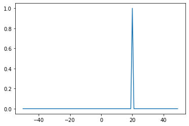
or, more generally, \[\begin{align} \int_{-\infty}^{\infty}{\delta(x-x_{0}) f(x) dx}=f(x_{0}) \tag{2} \end{align}\]
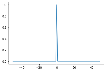
where \(f\) is an arbitrary function and \(x_{0}\) is a chosen value of \(x\) referred to as the center of the distribution. \(\delta(x)\) is often presented as a function defined such that \(\delta(x)=0\) for all \(x\neq0\) and \(\int{\delta(x) dx}=1\) (that is, a function that is zero everywhere except at the origin and has area 1) and that we can visualize as the limit of a unit area box function centered at the origin with width approaching 0 and height related to width by the \(\int{\delta(x) dx}=1\) condition.import scipy.signal as signal
import matplotlib.pyplot as plt
sample_count = 100
# Center of the distribution.
x_0 = 0
# The Dirac delta is also known as the Dirac impulse.
impulse = signal.unit_impulse(sample_count, (sample_count//2)+x_0)
plt.plot(np.arange(-50, 50), impulse)
import scipy.signal as signal
import matplotlib.pyplot as plt
sample_count = 100
# Center of the distribution.
x_0 = 20
impulse = signal.unit_impulse(sample_count, (sample_count//2)+x_0)
plt.plot(np.arange(-50, 50), impulse)
It is important to keep in mind, though, that \(\delta(x)\) is not a function, because no function satisfies the given conditions, and that a limit is not a function either.
Now, look at the condition that defines \(\delta(x)\) and observe that it picks out the value of \(f\) at any point \(x=x_{0}\) by integrating the product \(\delta(x-x_{0})f(x)\). The discrete counterpart of \(\delta(x)\), the unit impulse or unit sample \(\delta[x]\), \[\begin{align} \delta[x]=\begin{cases}1 & x=0 \\ 0 & x \neq 0 \\ \end{cases} \tag{3} \end{align}\]
has an analogous property: \[\begin{align} \sum_{k=-\infty}^{\infty}{\delta[x-k] f(k)}=f(x) \tag{4} \end{align}\]
This property is of great value to us and we’ll see later how it’s used to sample the value of \(f\) at regularly-spaced points of the domain. The remainder of this article uses the term Dirac delta to refer to \(\delta(x)\) and \(\delta[x]\).
The applications of Dirac delta distributions in rendering extend beyond sampling. For example, the directional distribution of a perfectly specular surface and, consequently, its BRDF, are Dirac deltas: only a single incident direction contributes to the reflected radiance in a given outgoing direction at a given point (which is to say that the outgoing direction determines the incident direction uniquely): \[\begin{align} f_{r}(p,\omega_{o},\omega_{i})=F_{r}(\omega_{r})\frac{\delta(\omega_{i}-\omega_{r})}{\vert \cos{\theta_{r}} \vert} \tag{3} \end{align}\]
where \(\omega_{r}\) is the specular reflection vector for \(\omega_{o}\) about the surface normal and \(\theta_{r}\) is the corresponding colatitude angle; in this case, \(\omega_{r}\) constitutes the center of the distribution.
Isotropic point lights are another example. These light sources have a Dirac delta distribution because they illuminate a given point only from a single direction (as opposed to area lights, which illuminate it from several directions).
The Dirac comb and sampling
The Dirac comb \(Ш_{T}(x)\), also known as impulse train or shah function, is a periodic distribution given by \[\begin{align} Ш_{T}(x)=T\sum_{k=-\infty}^{\infty}\delta[x-kT],\quad x\in\mathbb{R}, k\in\mathbb{Z} \tag{4} \end{align}\]
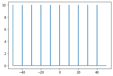
where \(T\) is the period. Observe that the Dirac comb is an infinite series of Dirac deltas, shifted by multiples of the period \(T\). To convince yourself (like I had to), evaluate \(Ш_{T}(x)\) at some \(x\in\mathbb{R}\): you’ll get 0 for any value of \(x\) that is not the center of one of the Dirac delta terms. This is, of course, because the function is periodic. And, like any periodic function, it satisfies \[\begin{align} Ш_{T}(x+T) &= T\sum_{k=-\infty}^{\infty}\delta[(x+T)-kT] \\ &= T\sum_{k=-\infty}^{\infty}\delta[x-(1-k)T] \\ &=\ Ш_{T}(x) \tag{5} \end{align}\]
The Dirac comb is so called because of the shape of its graph:import scipy.signal as signal
import matplotlib.pyplot as plt
sample_count = 100
T = 10
Fs = 1000
x = np.arange(-sample_count//2, sample_count//2, 1/Fs)
comb = np.zeros_like(x)
comb[::int(Fs*T)] = T
plt.plot(t, comb)
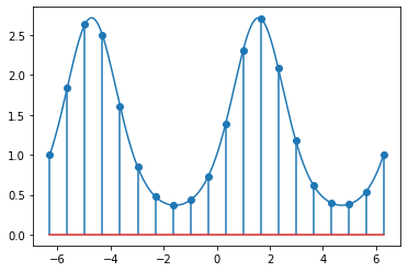
Observe that the centers of the Dirac delta terms are regularly-spaced across the domain of \(Ш_{T}\) (again, because it is periodic). This property along with \((4)\) allow us to sample the value of a function \(f\) at regularly-spaced sample points of its domain by multiplying it by \(Ш_{T}\): \[\begin{align} f(x) \cdot Ш_{T}(x) &= f(x) \cdot T\sum_{k=-\infty}^{\infty}\delta[x-kT] \\ &= T\sum_{k=-\infty}^{\infty}\delta[x-kT] f(x) \\ &= T\sum_{k=-\infty}^{\infty}\delta[x-kT] f(kT) \end{align}\]
Replacing \(f(x)\) by \(f(kT)\) has no effect on the summation, because the product \(\delta[x-kT]f(x)\) is 0 for all \(x\) except for \(x=kT\). With this substitution, it becomes clear that \(f(x) \cdot Ш_{T}(x)\) assumes the value of \(f(x)\) when \(x\) is a multiple of the period, and 0 everywhere else: \[\begin{align} f(x) \cdot Ш_{T}(x)=\begin{cases}f(kT) & x=kT, k\in\mathbb{Z} \\ 0 & x \neq 0 \\ \end{cases} \tag{3} \end{align}\]import matplotlib.pyplot as plt
import numpy as np
sample_count = 20
x = np.arange(-2.0*np.pi, 2.0*np.pi, 0.01)
y = np.exp(np.sin(x))
sample_x = np.linspace(-2.0*np.pi, 2.0*np.pi, sample_count)
sample_y = np.exp(np.sin(sample_x))
plt.plot(x, y)
plt.stem(sample_x, sample_y, use_line_collection=True)
plt.show()
Ideal sampling and reconstruction
To sample the value of a function \(f\) at regularly-spaced sample points of the domain, the function is multiplied by an impulse train function or shah \(III_{T}(x)\): \[\begin{aligned} III_{T}(x)f(x) \end{aligned}\]
where \[\begin{aligned} III_{T}(x)=T\sum_{k=-\infty}^{\infty}\delta[x-kT] \end{aligned}\]
and \(T\) is the period or sampling rate. Observe that the impulse train \(III_{T}(x)\) is an infinite series of Dirac deltas, shifted by multiples of the period \(T\). As we saw earlier, integrating the product of \(f(x)\) and the Dirac delta \(\delta[x-x_{0}]\) over a continuous domain yields \(f(x_{0})\); similarly, summing up this product over a discretized domain yields \(f(x_{0)\): \[\begin{aligned} \sum_{k=-\infty}^{\infty}{\delta[x-x_{0}] f(x)}=f(x_{0}) \end{aligned}\]