Oren-Nayar Reflectance Model
This post is part of a series of posts I’m writing about the CPBRT renderer, an implementation of Pharr, Jakob and Humphrey’s PBRT.
The Oren-Nayar reflectance model is a generalization of Lambert’s reflectance model for diffuse reflection. Unlike Lambert’s, which models perfect diffuse reflection from smooth surfaces, Oren-Nayar’s models reflection from surfaces of varying degrees of roughness realistically.
In their paper titled Generalization of Lambert’s Reflectance Model (pdf), Oren and Nayar observed that the microgeometry of a rough surface influences our perception of its appearance, making it look brighter as the viewing direction approaches the incident illumination direction. They also noted that Lambert’s model didn’t capture this effect and so they set out to model it properly.
The Lambert reflectance model
A Lambertian surface is an ideal diffuser that reflects incident radiance equally in all directions independently of the viewing direction and the proximity of the camera to the surface: no matter where the camera is, a Lambertian surface appears equally bright from all viewing directions and distances. Oren and Nayar claim that no diffuse surface in the real world reflects light that way and attribute Lambert’s poor approximation of the phenomenon to the fact that it doesn’t factor in the complex effects that the microgeometry of a rough surface has on incident light.
The reason why Lambertian reflection is a poor approximation is that it doesn’t take the roughness of the surface into account. In fact, its hemispherical-directional reflectance \(\rho_{dh}\) is a constant spectral value (commonly called the diffuse color \(R\)) and so is its BRDF: \[\begin{aligned} R &= \rho_{dh}(\omega_{i}) \\ &= \int_{\omega_{o} \in H^{2}(n)}{f_r(p,\omega_{i},\omega_{o})\ \vert \cos{\theta_{o}}\vert\ d\omega_{o}} \\ &= f_r(p,\omega_{i},\omega_{o})\int_{\omega_{o} \in H^{2}(n)}{\vert \cos{\theta_{o}}\vert\ d\omega_{o}} \\ &= f_r(p,\omega_{i},\omega_{o})\int^{2\pi}_{\phi_{i}=0}{\int^{\pi/2}_{\theta_{i}=0}{\vert \cos{\theta_{i}}\vert\ \sin{\theta_{i}}\ d\theta_{i}}\ d\phi_{i}} \\ &= f_r(p,\omega_{i},\omega_{o})\ \pi \\ \\ &\iff \\ \\ f_r(p,\omega_{i},\omega_{o}) &= \frac{R}{\pi} \end{aligned}\]
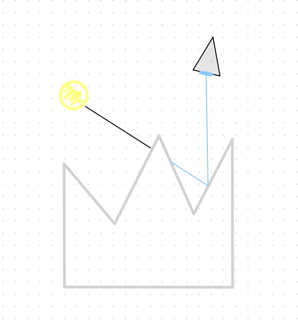
Observe that nowhere in this expression does the viewing direction or the distance to the camera appear. Consider then a rough surface that the camera looks at from up close and from some distance:
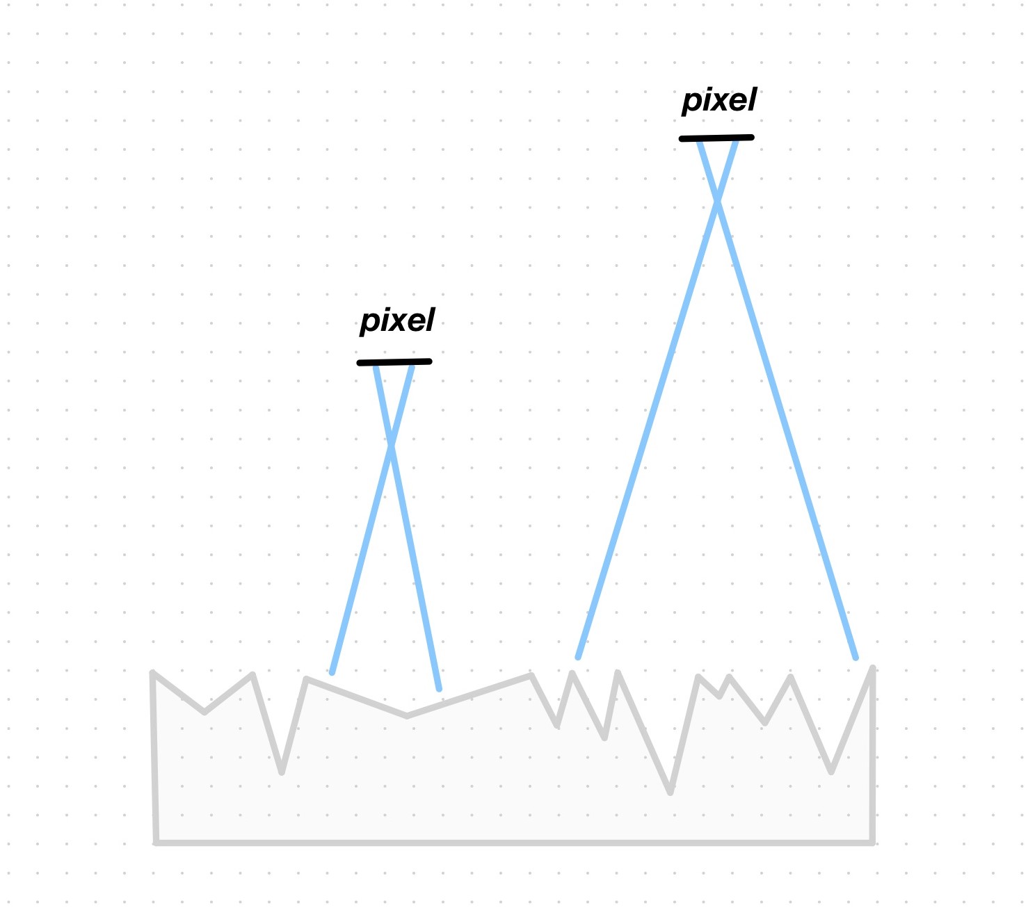
The directional distribution of the example surface can’t possibly be modelled by a constant: the intricacies of the geometry of the surface warrant a reflection model that acknowledges (1) that the orientation and slope of the surface vary at the microscopic level across different points and (2) that a nonconstant relation exists between these differences and the position of the camera that determines the perceived brightness. We’ll soon see how Oren-Nayar factors in these intricacies.
The Oren-Nayar reflectance model
Oren-Nayar models surfaces of varying degrees of roughness as collections of long, symmetric V-shaped cavities. V-shaped cavities are just one of many microfacet models out there that model the scattering of light from rough surfaces statistically. In particular, Oren-Nayar takes the V-cavities microgeometries of Torrance and Sparrow (pdf) and describes them with a probability distribution of facet-slope per unit area parametrized by the standard deviation of the slope angle.
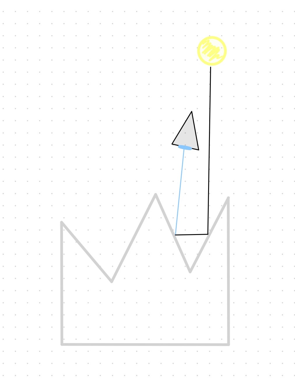
To understand why the perceived brightness changes across the surface and as the viewing direction changes, it’s essential to understand the geometrical setting:
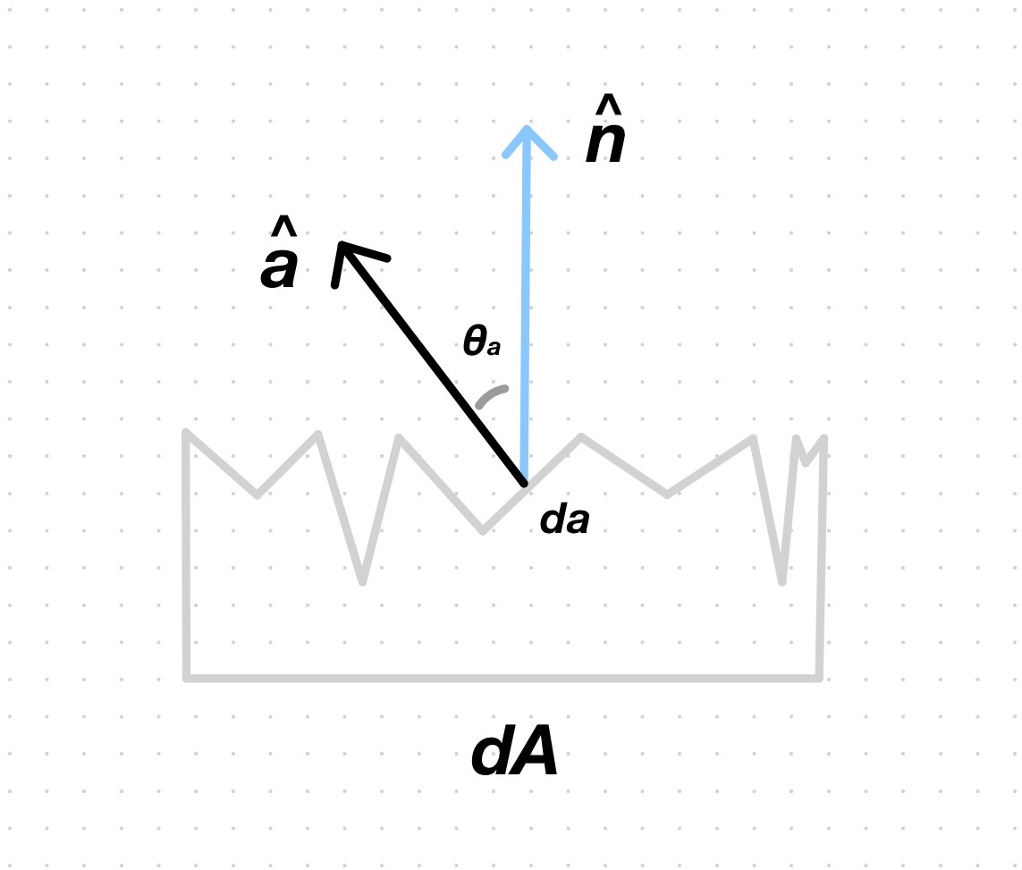
a V-cavity is modelled as a pair of planar facets that face each other; the facets of a given V-cavity have equal area, denoted \(da\), which may differ across V-cavities; \(da\) is assumed to be much smaller than the area differential \(dA\) that is imaged by a single pixel, so multiple V-cavities will be contained by a single one;
each facet is further characterized by a normal vector \(\hat{a}\) whose direction is given by the spherical coordinate \((\theta_{a},\phi_{a})\), where the polar angle \(\theta_{a}\) gives its slope and the azimuth angle \(\phi_{a}\) gives its orientation; if we let \(\hat{n}\) denote the normal vector of the surface, then we refer to \(\hat{n}\) as the macronormal and \(\hat{a}_{k}\) as a collection of facet micronormals;
and because a given ray of light will ultimately hit facets, the reflectance of each one is assumed to be Lambertian.
With such a representation in mind, we can begin to understand the effects that the geometry of a rough surface has on incident light. First, assume that all the V-cavities of the surface have a delta distribution of slope and orientation. Now imagine the cross-section of one such surface; place the camera above it and oriented in a way such that its line of sight is parallel to the length of the cross-section; and place a distant light source above the surface, fixed somewhere to the right. We’ll observe that
there’ll be a brightness disparity between the 2 facets of each of the V-cavities: the ones to the left will receive more light than the ones on the right; the surface will then be perceived bright when looked at from the right and dark from the left; we can then infer that the perceived brightness of the surface will vary between these 2 poles as the camera rotates from one side to the other;
since the area \(da\) of the facets of a V-cavity of interest may be smaller than the areas of those of neighboring V-cavities, the facet of the V-cavity of interest that faces the camera may be partially or completely occluded and invisible to it; this effect is called masking;
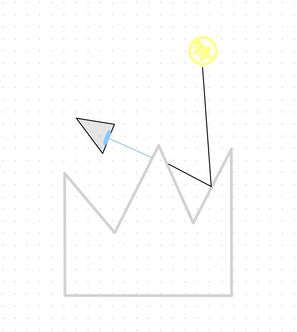
- if, on the other hand, the camera does see the facet of the V-cavity of interest, but the line between the light source and the facet is interrupted by a (taller) neighboring V-cavity, it will be dark; this effect is called shadowing;
- and depending on the direction of incidence and the slope of the facet of the V-cavity of interest, light may bounce toward the other facet of the V-cavity and escape it only after a series of interreflections.
In this example, we assumed that the surface had a delta distribution of facet slope and orientation. By that, we meant that the fraction of the surface (macro) area differential, \(dA\), that is covered with microfacets with a certain normal \(\hat{a}=(\theta_{a},\phi_{a})\) possessed a delta distribution. In the general case, though, Oren and Nayar give a normal distribution with mean \(\mu_{\theta}=0\) and a configurable standard deviation \(\sigma_{\theta}\) to the microfacet slope, and refer to it as the slope-area distribution of the surface, \(P(\theta_{a};\mu_{\theta},\sigma_{\theta})\); whereas they give a uniform distribution to the orientation \(\phi_{a}\). The reflectance and outgoing radiance equations, as well as the BRDF, are thus developed for surfaces with isotropic roughness in mind (i.e. if you rotate the surface about the (macro) normal at one point, the reflectance distribution doesn’t change), but the authors claim that this model encompasses surfaces with anisotropic roughness, too; I don’t know why or how, though.
With \(P(\theta_{a},\phi_{a},\sigma_{\theta})\) as the directional distribution factor of the scattering equation, the total outgoing radiance reflected by the surface is given by \[L_{o}(\theta_{o},\phi_{o},\theta_{i},\phi_{i},\sigma_{\theta})=\int^{\pi/2}_{\theta_{a}=0}{\int^{2\pi}_{\phi_{a}=0}{P(\theta_{a},\phi_{a},\sigma_{\theta})\ L_{op}(\theta_{a},\phi_{a})\ \sin{\theta_{a}\ d\phi_{a}\ d\theta_{a}}}}\]
where \(L_{op}(\theta_{a},\phi_{a})\) denotes the projected radiance of a facet with normal \(\hat{a}=(\theta_{a},\phi_{a})\) and gives its contribution to the total radiance reflected by the surface. Observe that \(L_{o}\) integrates over the hemisphere of directions, that is, over every possible facet normal \(\hat{a}\), and that the radiance \(L_{op}(\theta_{a},\phi_{a})\) reflected by facets of a given normal \(\hat{a}\) is weighted by the reflectance distribution \(P(\theta_{a},\phi_{a},\sigma_{\theta})\). Contributions to the total reflected radiance are thus proportional to the fraction of the surface that is covered with microfacets with normal \(\hat{a}\).
Now, recall that for a rough surface to be modelled realistically, we need to account for the effects of masking, shadowing, and interreflection. These effects are encapsulated in the projected radiance factor \(L_{op}(\theta_{a},\phi_{a})\) in the forms of a geometric attenuation factor, GAF, and an interreflection factor, IF. The GAF is the ratio of the facet area that is both visible (not masked) and illuminated (not shadowed), to the total area \(da\) of the facet, and has the effect of reducing the projected radiance from direct illumination that the facet reflects; the attenuated projected radiance is denoted by \(L^{1}_{op}(\theta_{a},\phi_{a})\). The IF, on the other hand, has the effect of increasing the projected radiance of the facet by the amount of radiance that the opposite companion facet of the V-cavity reflects onto it, and has the form of a separate term \(L^{2}_{op}(\theta_{a},\phi_{a})\). The projected radiance reflected by a facet is thus given by \[L_{op}(\theta_{a},\phi_{a})=L^{1}_{op}(\theta_{a},\phi_{a})+L^{2}_{op}(\theta_{a},\phi_{a}).\]
which, to reiterate, gives the contribution of a single facet to the total radiance reflected by the surface. Unfortunately, the total outgoing radiance \(L_{o}(\theta_{o},\phi_{o},\theta_{i},\phi_{i},\sigma_{\theta})\) and the BRDF are not easy to evaluate, so they aren’t used in practice. PBRT (and CPBRT consequently) use the following approximation of the BRDF instead: \[\begin{aligned} f_{r}(\theta_{o},\phi_{o},\theta_{i},\phi_{i}) &= \frac{R}{\pi}(A+B\max(0,\cos(\phi_{i}-\phi_{o}))\sin{\alpha}\tan{\beta}) \\ &= \frac{R}{\pi}(A+B\max(0,\cos{\phi_{i}}\cos{\phi_{o}}+\sin{\phi_{i}}\sin{\phi_{o}})\sin{\alpha}\tan{\beta}) \end{aligned}\]
where \[\begin{aligned} A &= 1-\frac{\sigma^{2}}{2(\sigma^{2}+0.33)} \\ \\ B &= \frac{0.45\sigma^{2}}{\sigma^{2}+0.09} \\ \\ \alpha &= \max(\theta_{i},\theta_{o}) \\ \\ \beta &= \min(\theta_{i},\theta_{o}) \end{aligned}\]
and \(R\) is the albedo or Lambertian diffuse color of the facet. Oren and Nayar claim that this approximation is accurate enough for arbitrary roughness and angles of incidence and reflection, and that it obeys Helmholtz’s reciprocity principle (i.e. for all pairs of directions \((\theta_{i},\phi_{i})\) and \((\theta{o},\phi{o})\), \(f_{r}(\theta_{o},\phi_{o},\theta_{i},\phi_{i})=f_{r}(\theta_{i},\phi_{i},\theta_{o},\phi_{o})\)). This expression trades accuracy for computability, so be warned; the loss of accuracy comes mainly from discarding the interreflection term.
As mentioned at the beginning, the Oren-Nayar reflectance model is a generalization of Lambert’s. This is the case in both the theoretical and precise model and the approximation. In particular, if we subtitute \(A=1\) and \(B=0\) in the approximation, we obtain the BRDF of the Lambert model: \[\begin{aligned} f_{r}(\theta_{o},\phi_{o},\theta_{i},\phi_{i}) &= \frac{R}{\pi}(1+0\max(0,\cos(\phi_{i}-\phi_{o}))\sin{\alpha}\tan{\beta}) \\ &= \frac{R}{\pi} \end{aligned}\]
Implementation and results
Commit d9fd4fd added the OrenNayarReflection class to CPBRT, which implements the Oren-Nayar reflectance model using the approximation to the theoretical BRDF.
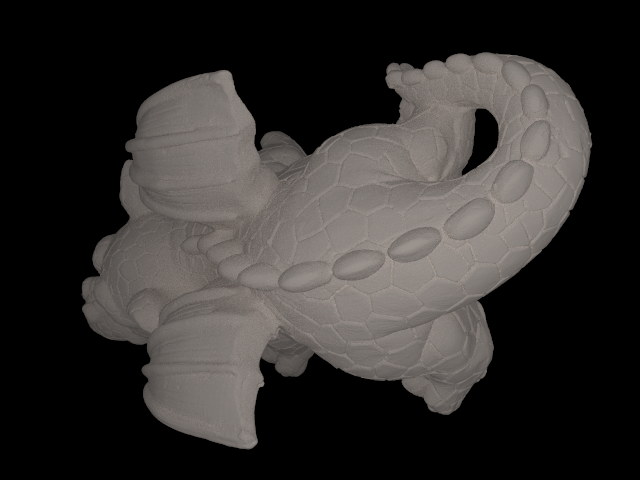
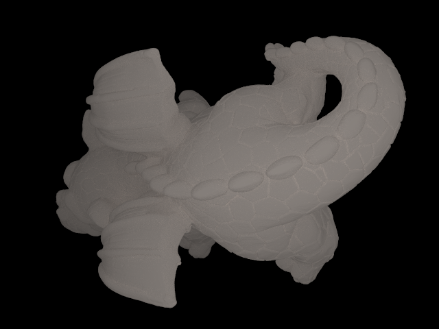
The following 2 renders feature the dragon triangle mesh by Christian Schüller with a matte material that uses (1) the Lambert BRDF and (2) the Oren-Nayar BRDF with \(\sigma_{\theta}=20°\), illuminated by one point light located at the camera:
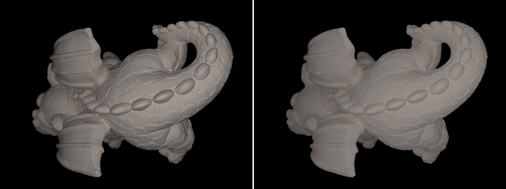
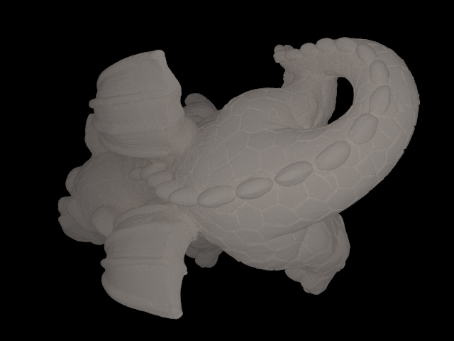
I’m not great at describing the differences, but I would say that both exhibit at least the main characteristics that the clay cylindrical vases in the paper have (see Figure 22): in the Lambert one, brightness declines gradually and towards the boundary of the mesh as the surface normals begin to point away from the light source; whereas in the Oren-Nayar one, brightness remains pretty much constant across the surface. In general, brightness increases with \(\sigma_{\theta}\):


For a deeper (and correct) understanding of the model, I refer the interested reader to Physically Based Rendering: From Theory To Implementation, by Pharr, Jakob and Humphrey, 2016.