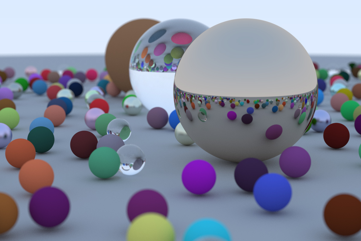
First ray tracer: Ray Tracing in One Weekend
Ray Tracing in One Weekend by Peter Shirley must be the best end-to-end introduction to ray tracing out there: it’s accesible enough for beginners, but sufficiently rigorous to lead to a correct implementation.
This post isn’t a summary of the book; the 1000 Forms Of Bunnies blog does a much better job at that. This post captures my understanding of the essential concepts, examines some of the equations a little bit more closely, and presents renders of failed attempts. Of course, reading the original source is your best option.
The source code is available in my repo github.com/carlos-lopez-garces/ray.
Intro
Indirect lighting is one of the most important effects implemented by ray tracing. Not only will objects illuminated directly by a light source have their color revealed, also those that are reached by light that bounces off of the surface of others or that passes through those others.
Ray tracing algorithm
The ray tracing algorithm samples the radiance of light that light sources emit and that travels and bounces around the scene until it reaches the camera. At a very high level, the ray tracing algorithm goes something like this:
1. Shoot a ray from the camera to a pixel.

2. Trace the ray as it bounces from surface to surface until it reaches a light source
   or some maximum number of bounces, or until it escapes the scene. At each intersection
   point, sample the directional distribution of the surface to determine the direction
   of the bounce.

3. Sample the light source and trace the ray back along the same path until it reaches
   the camera, keeping the spectral value of the radiance carried by the ray in a color
   variable. At each intersection point, let the material of the surface determine the
   spectral distribution of the reflected or refracted light.

4. Assign the computed color to the pixel.
This, of course, is an oversimplification that omits important steps.
Rays
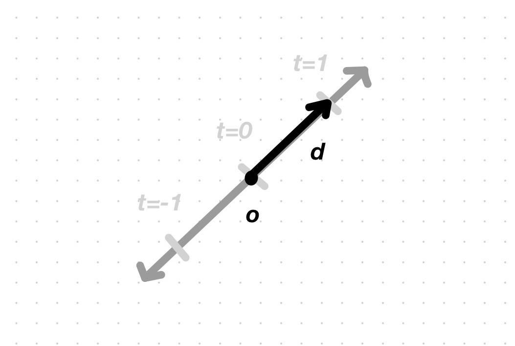
A ray is a vector-valued function \(\pmb{r}(t) = \pmb{o} + t\pmb{d}\), where \(\pmb{o}\) is the origin point of the ray, \(t\) is the parameter and \(\pmb{d}\) is the direction vector. The function’s value at each value of the parameter is a point along the ray.
Linear interpolation
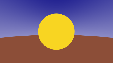
The first image that you’ll render is a gradient from one color to another; a linear interpolation, or lerp, of 2 colors, e.g. white at 0.0 and sky blue at 1.0, and the values in between blend the 2 of them. The value of the \(t\) parameter is determined by the pixel’s \(v\) coordinate: \[\pmb{blendedColor} = (1-\pmb{t}) \cdot startColor + \pmb{t} \cdot endColor\]

Ray-sphere intersection
Scenes in book 1 consist of spheres exclusively, so it’s necessary to know how to intersect them.
The equation of a sphere centered at the origin is \(x^2+y^2+z^2=R^2\):
Any point \((x,y,z)\) that satisfies the equation lies on the surface of the sphere.
Any point \((x,y,z)\) that satisfies the inequality \(x^2+y^2+z^2<R^2\) is inside the sphere.
When the sphere is not centered at the origin, but at a point \(C\), the equation becomes \((x-C_x)^2+(y-C_y)^2+(z-C_z)^2=R^2\).
The point \(p'=(x-C_x, y-C_y, z-C_z)\) is the translation of point \(p=(x, y, z)\) of the original sphere to the origin. This translation can be expressed in terms of vectors: \(P'=P-C\).
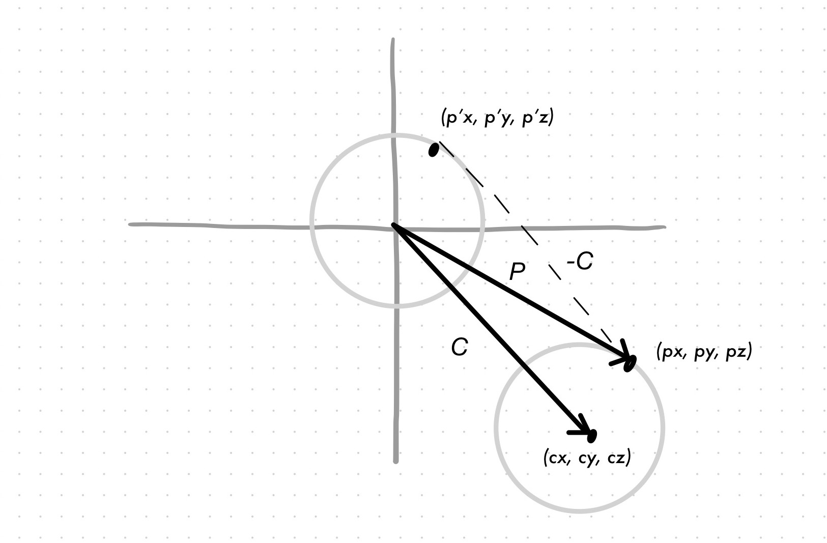
In vector form, the equation of the sphere becomes \((P-C)\cdot(P-C)=R^2\). Recall that the dot product is the sum of the component-wise multiplication. In this case, it is the sum of the square of each component of vector \(P-C\), which, as seen in the picture above, yields a point on the sphere centered at the origin when that point satisfies the equation.
Now, recall that a ray is a vector-valued function \(\pmb{r}(t) = \pmb{o} + t\pmb{d}\). We want to know if the ray intersects the sphere, i.e. we want to know if there is a \(t\) such that \(\pmb{r}(t)\) satisfies the equation of the sphere: \((\pmb{r}(t)-C)\cdot(\pmb{r}(t)-C)=R^2\).
When expanding and regrouping the equation, it is revealed that the equation is quadratic: \[\begin{aligned} (A+tB-C)\cdot(A+tB-C) &= R^2 \\ \{B \cdot Bt^2\} + \{2B \cdot (A-C)t\} + \{(A-C)\cdot(A-C)-R^2 \} &= 0 \implies ax^2+bx+c=0 \end{aligned}\]
where we can see the quadratic, linear, and constant terms.
A quadratic equation may have 0 roots (when no \(t\) satisfies it), 1 root (when 1 \(t\) satisfies it) or 2 roots (when 2 \(t\)s satisfy it):
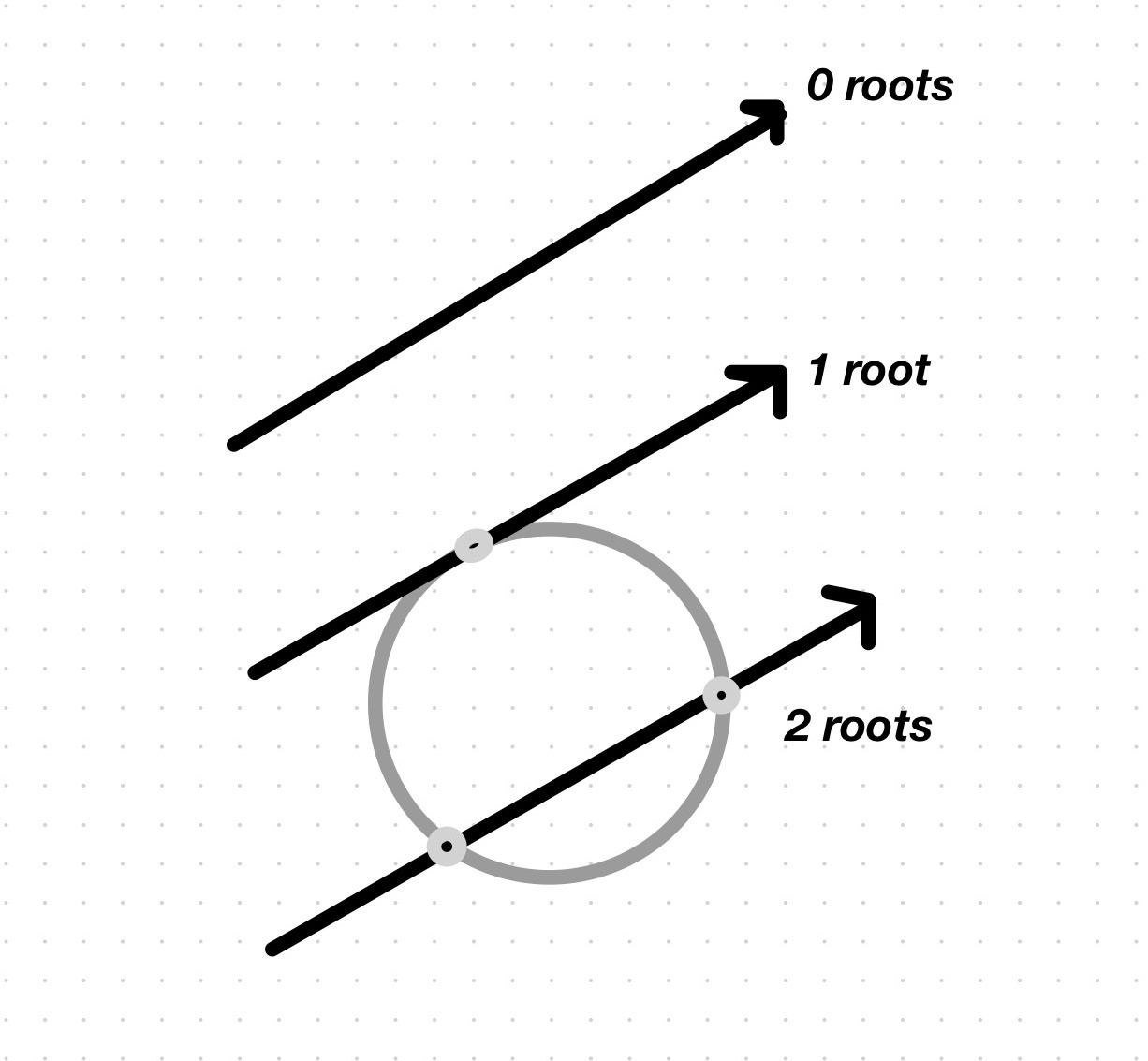
The roots are found by solving the quadratic formula: \[\begin{aligned} x &= \frac{-b\pm\sqrt{b^2-4ac}}{2a} \\ t &= \frac{-\{2B \cdot (A-C)\}\pm\sqrt{\{2B \cdot (A-C)^2\} - 4(B \cdot B)\{(A-C) \cdot (A-C) - R^2\}}}{2(B \cdot B)} \end{aligned}\]
But we are not interested in the actual intersection point, only in whether there is one. The discriminant’s sign tells you the number of roots: none if negative (the square root doesn’t give a real number), 1 if 0 (the square root of 0 is only 0), 2 if positive (the square root of a positive number). (There is so much more to the discriminant.)
Surface normals
If we want to shade the sphere, we’ll need to compute the intersection points, by substituting \(t\) in the ray vector function \(\pmb{r}(t) = \pmb{o} + t\pmb{d}\) with the values of the roots. The root that yields the closest intersection point to the camera is the one that the ray should use to sample the sphere (the other one will be occluded by the sphere itself).
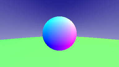
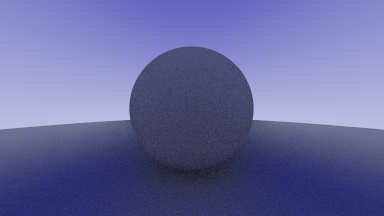
Here, the color sampled by each ray is given by the normal of the surface:
With unit vector normals
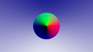
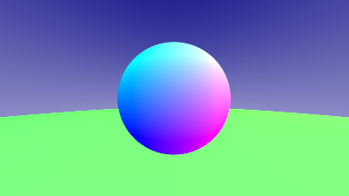
With normal
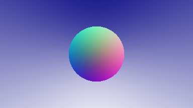
It looks dark. The author adds a (0.5, 0.5, 0.5) gray to brighten it.
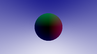
Brightened up with gray
Front faces and back faces
For certain kinds of objects, it’s important to be able to tell if, at a given hit point, the ray is coming from inside the surface or outside the surface. For most opaque surfaces, the only hit point that matters is the one where the ray is coming from outside the surface. In some translucent objects, though, like balls of glass, the other hit point also matters.
One way to tell is to look at the relative directions of the normal and the ray: if they go in opposite directions about a line tangent to the surface, then the ray is incoming and comes from outside the surface; if they go in the same general direction about the tangent line, the ray is outgoing and comes from inside the surface. If the angle between the normal and the ray is between \(90°\) and \(270°\) (\(\pi/2\) and \(3\pi/2\)), the ray is on the other side of the tangent line; if the angle is between \(270°\) and \(90°\), the ray is on the same side of the tangent line as the normal.
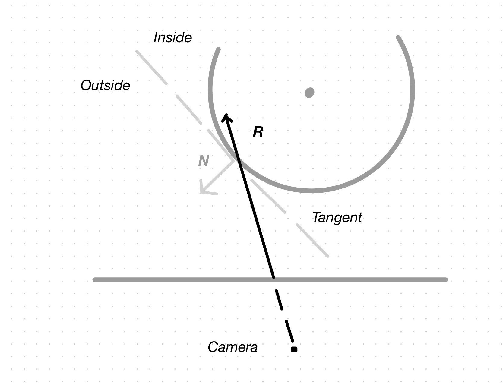
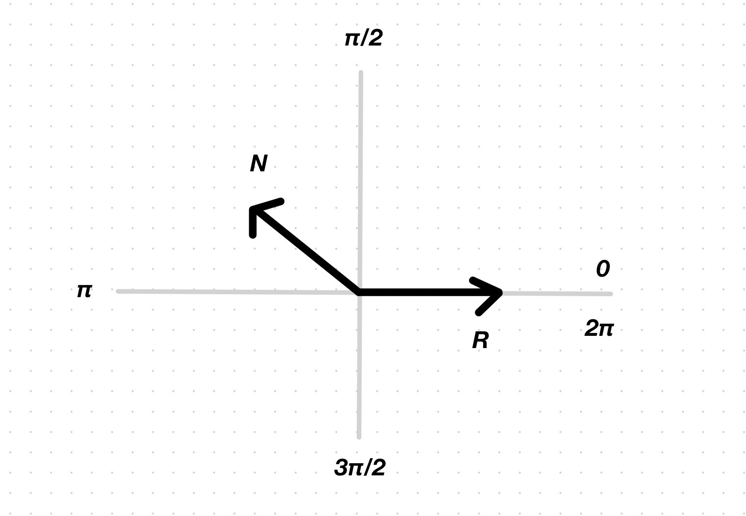
As always, we use \(r(t) \cdot N\) to compute the cosine of the angle between the ray and the normal. If we divide the plane in 4 quadrants, aligning the horizontal axis with the ray vector (and forgetting about the tangent line for a second), we see that the cosine is negative in quadrants II and III, and positive in quadrants IV and I. The sign thus tells us the side the ray is coming from.
Antialiasing
Aliasing is the result of sampling at a rate that doesn’t match the frequency content of the scene. Here, aliasing is lessened by averaging multiple samples inside each pixel.
One sample per pixel
100 samples per pixel, average color
When using a single sample per pixel, you are typically using the color of the object intersected by a ray that passes through one of the corners of the pixel or by its center.
For a given pixel, our antialiasing solution samples the scene with multiple rays, each passing through the pixel at random \((u, v)\) offsets. The colors sampled by these rays are then averaged to produce the final color for the pixel.
Multiple random samples of a single pixel
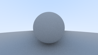
Diffuse materials
We now turn our attention to the first reflection model implemented in book 1: diffuse.
Diffuse objects reflect light in random directions. Light that bounces off a surface has its direction randomized; the fact that the direction of the view ray doesn’t influence the ray’s outgoing direction makes this model an omnidirectional scattering one.
Diffuse objects that don’t emit light merely take on the color of their surroundings, but they modulate it with their own intrinsic color. Some light may be absorbed by the object too (dark surfaces absorb more light than light surfaces).
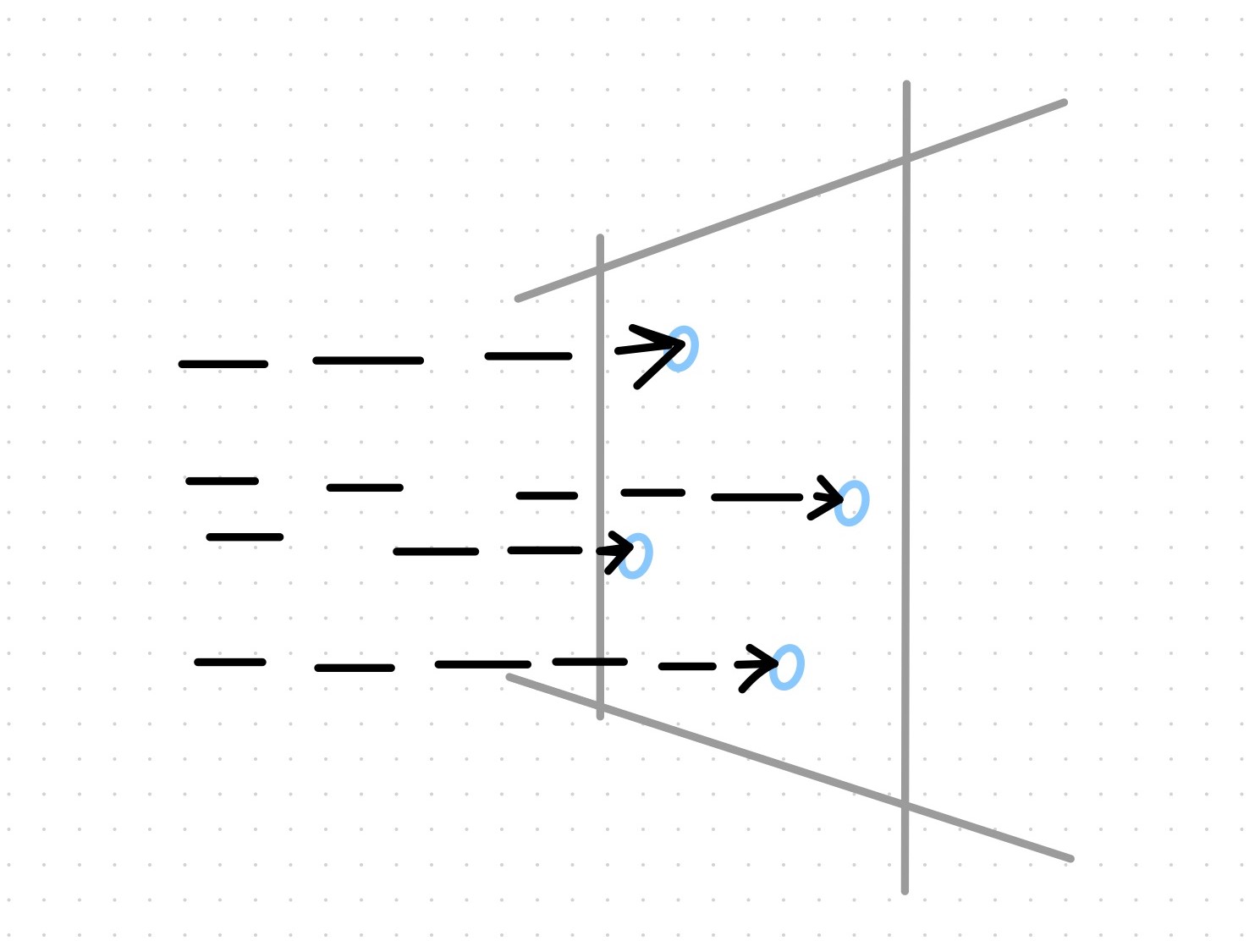
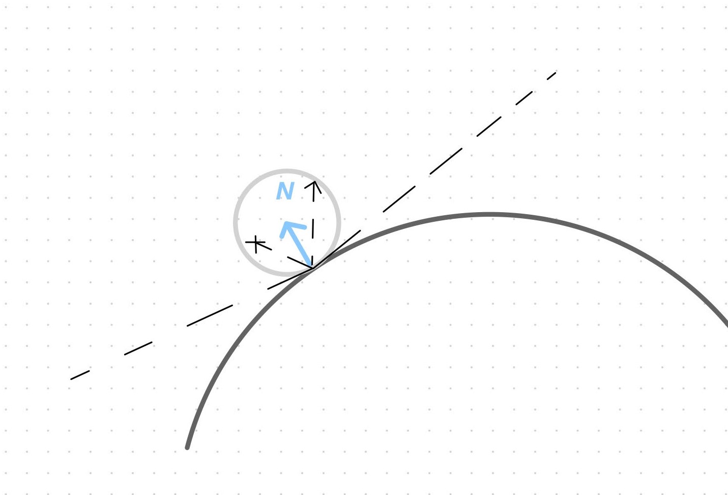
Random scattering
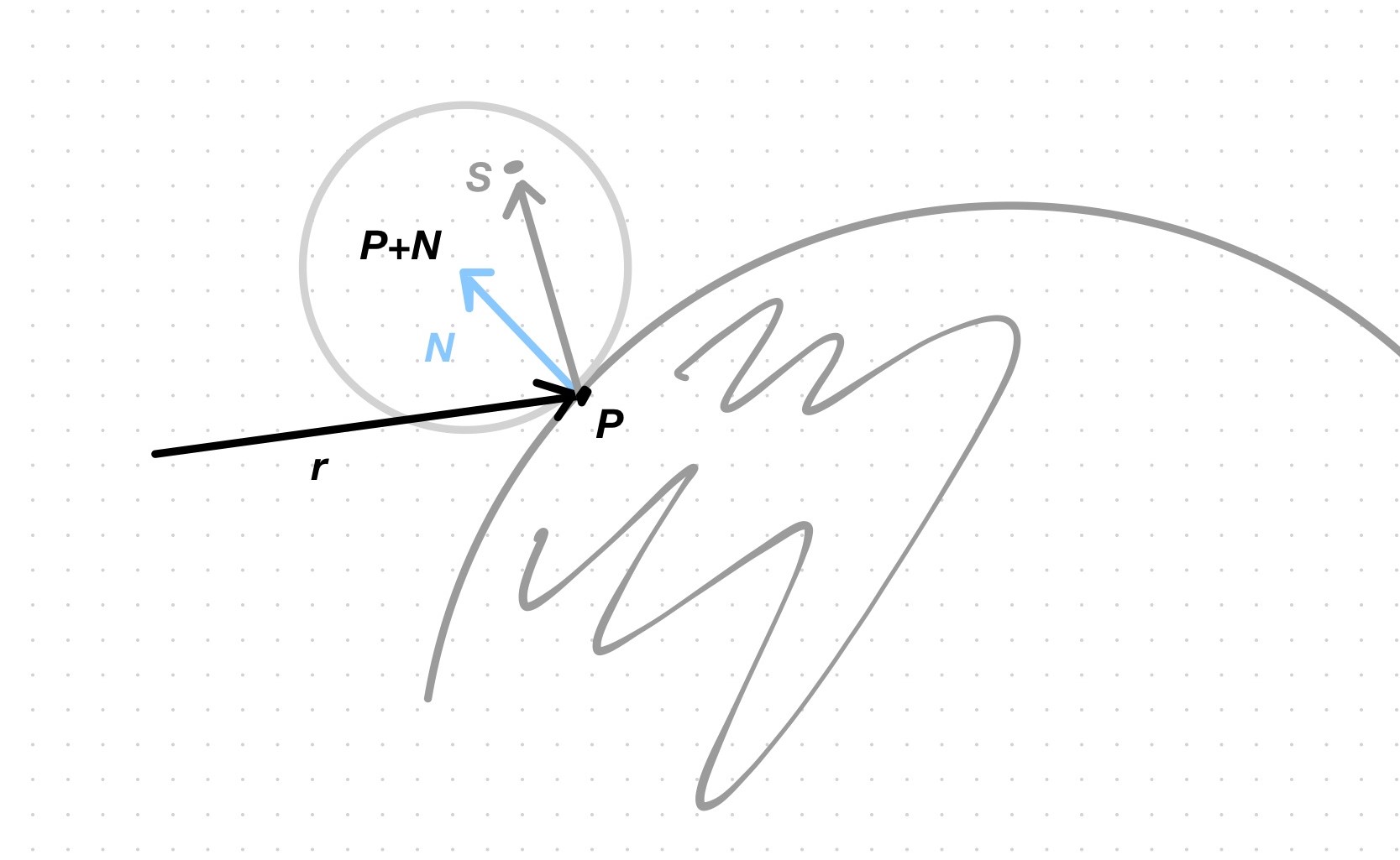
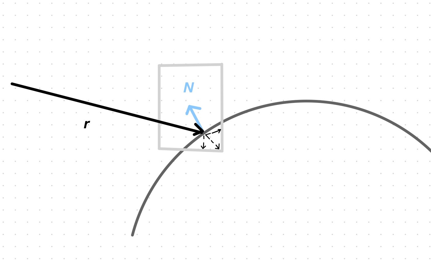
This is how you randomize the bounce of the ray: place a unit radius sphere tangential to the surface hitpoint \(p\). This sphere has its center at \(p + N\), when the ray comes from outside the surface, or \(p - N\), when it comes from inside. Since the normal is a unit vector, the sphere has a unit radius. Now pick a random point \(s\) on the surface of the sphere and send a ray from the hitpoint \(p\) to the random point \(s\) to sample the color of the object that it intersects. Finally, mix this color with the object’s color.
Ray bounces in the direction of a random point on the unit sphere
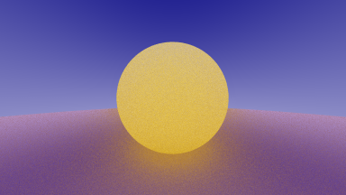
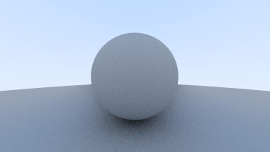
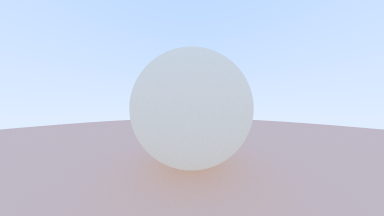
My first attempt: one bounce ray per ray, 100 rays per pixel, objects have an intrinsic color
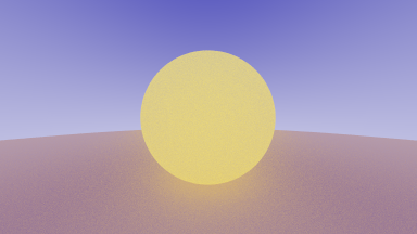
Same as above, but color is multiplied by an absorption factor of 0.5 (called diffuse reflectivity coefficient):
objects absorb 50% of the radiance and don’t reemit it
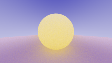
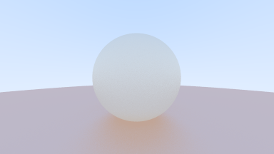
Gamma corrected, \(\gamma=2\)
(I was getting this, but it’s a mistake, I was halving only the intrinsic color and adding it to the bounce’s color, instead of halving the sum.)
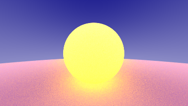
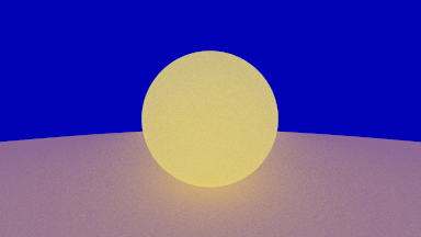
(Changed background to plain blue. This made me realize that the formerly white bottom half of the gradient doesn’t contribute much to the colors of the objects. A ray headed or bouncing in the direction of the bottom half is bound to intersect the ground instead. So pretty much all rays that bounce and don’t hit an object end up sampling the blue upper half.)
Zero bounces, for reference
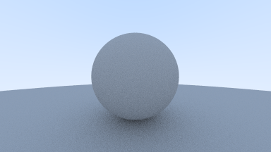
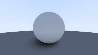
Increase the number of bounces by recursively tracing the ray until it doesn’t hit anything (at which point it’ll sample the background) or a maximum number of bounces is reached (at which point the sample is black so as not to contribute), halving the color each time it bounces (all objects in this example scene absorb half the energy of the ray on each bounce).
The color of a hitpoint whose ray bounces too many times (without ever going off into the background) tends to black: it’s more evident when objects don’t have an intrinsic color, and the only colors to sample from are the background’s and the black of a ray that bounces past the maximum limit.
The area near the point of contact of the sphere and the ground is interesting: a faint shadow forms because rays there are very likely to keep bouncing between the 2 surfaces, darkening the ray’s sample by absorption (-50% per bounce in this scene).
I originally thought that most of the rays in this area must be sampling the back faces (the interior) of the sphere but I was wrong. I thought this because I was thinking that the origin point of the bounce was the center of the tangential unit sphere, which may indeed lie in the interior of the scene’s sphere; but the origin is really on the ground surface.
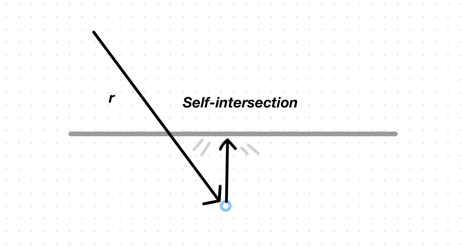
It’s very subtle, but the render suffers from shadow acne: the reflected ray intersects its origin surface because its origin is not exactly \(t=0\) but some floating point approximation that causes it to be below the surface sometimes.
The ray will bounce off its origin surface and this extra bounce will half the origin point’s color, causing it to appear darker than the surrounding points.
The cause of shadow acne
As to how to select the bounce’s direction without sampling a directional distribution of the surface, you can do it in several ways:
- Axis-aligned unit cube: bounce in the direction of a random point on the surface of a unit cube centered at a distance of 1 unit from the hit point in the direction of the normal. The problem of doing it this way is that the cube may penetrate the surface at certain hit points and the sampled point may be inside the surface; the bounce ray would then head towards the interior of the surface, and once inside, the ray can’t escape: it will keep bouncing until it reaches the limit, its color tending to black with each bounce.
Tangential unit sphere: all rays bounce away from the surface.
Note that all bounces are contained by a cone and that no ray will ever bounce outside this cone; I don’t know what the consequences of that are, all I know is that the scattering angle computed by the Lambertian model (a mathematical approximation of diffuse scattering) tends to be close to the angle of the normal (i.e. the majority of rays are scattered with angles that approximate the normal, while fewer are scattered at shallow angles w.r.t. to the surface). So this simpler unit sphere scattering approximation is similar to Lambert in this sense.
Another thing to note is that the scattering angle is independent of the ray’s incidence angle in this model. I don’t know if that’s OK.
- Cylinder of length 1: the problem with sampling a unit sphere is that the resulting direction is biased towards the normal and that grazing angles are produced with very low probability. Sampling a cylinder produces a more uniform result. The result is evident near the contact point of the spheres: it is darker in the unit sphere case because more rays will bounce in the direction of the normal and are bound to hit the other surface and bounce back, and with each bounce there’s more absorption; it is lighter in the cylinder case because more rays escape towards the background at grazing angles, without hitting the other surface. This is supposed to be the correct way to render diffuse surfaces according to the Lambert model.
- Hemisphere of tangential unit sphere: sample the unit sphere that is tangential to the surface at the hit point and reverse the direction of the resulting vectors that sample the lower hemisphere.
Lambert material
Lambert is a physically-correct model for diffuse materials.
Attenuation can be implemented in 2 ways:
- By absorbing completely a fraction of the rays (with a given probability) and not
  attenuating the ones that do get scattered/reflected.
- By scattering/reflecting all the rays, but diminishing their color.
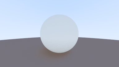
The concept of albedo enters the picture. The albedo of a surface is the proportion of incident light or radiance that it reflects.
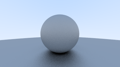
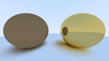
Small sphere with albedo (0.5, 0.5, 0.5)
Big sphere with albedo (0.2, 0.2, 0.2)
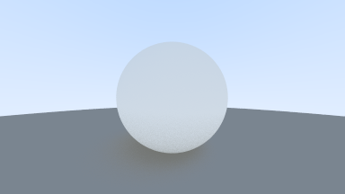
With different base colors
With the same base colors
Metal/mirror material
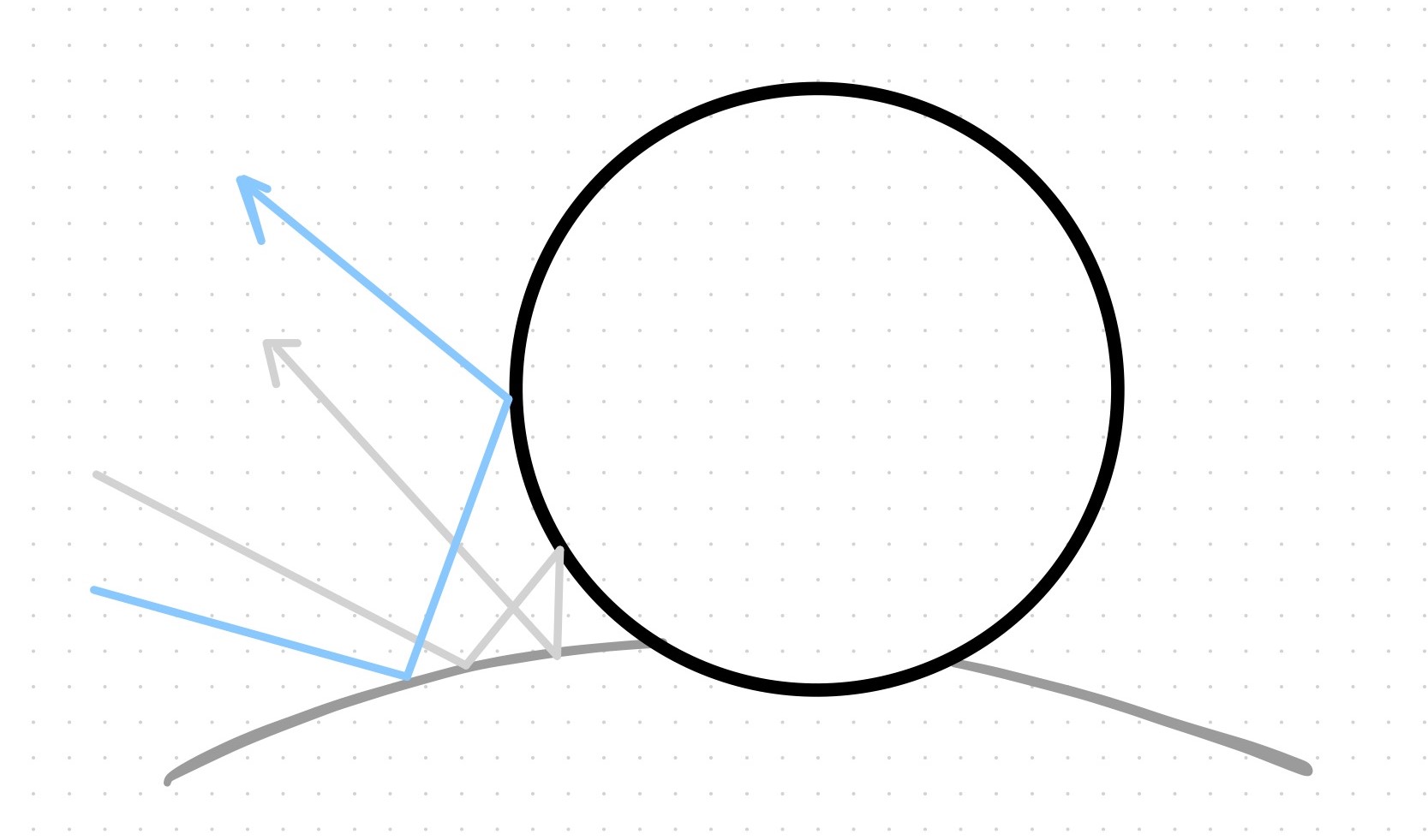
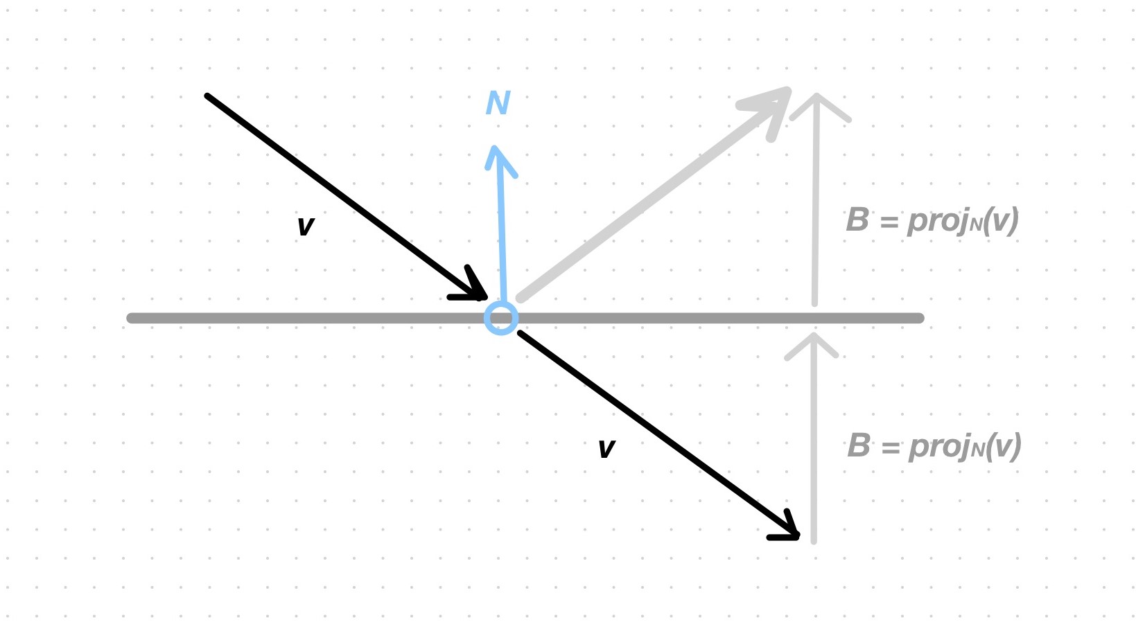
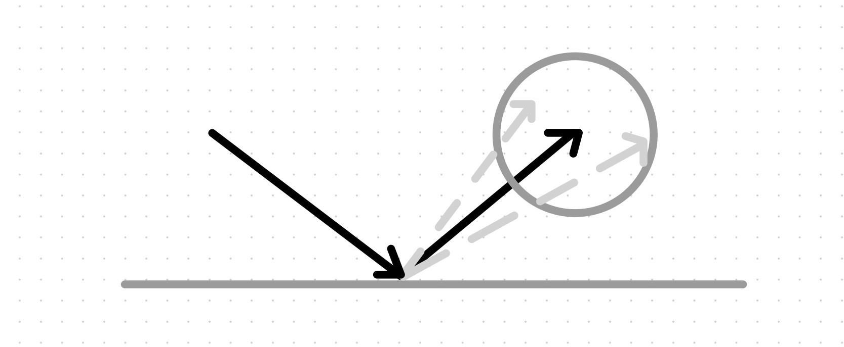
A perfectly smooth reflective surface, like a mirror or smooth metal, reflects rays at the same angle of incidence.
\(v \cdot N\) is the length of the scalar projection of \(v\) onto \(N\), depicted here as \(B\). \(B\) can also be seen as the unit vector \(N\) scaled by \(v \cdot N\) and thus as the vector component of \(v\) that goes in the direction of \(N\). How is the vector of the reflected ray computed? Place \(v\) at the hit point; it will point into the surface. Add \(B\) to it; the result \(v+B\) is a vector that is tangential to the surface and perpendicular to the normal \(N\). Add \(B\) again; the result is a vector that forms a right angle with \(v\).
Wrong reflection vector computation


Correct reflection vector computation
Correct, albedo gives it its color
Randomize the tip of the reflected ray by sampling a point on the surface of a sphere centered at the tip. This has the effect of making the reflection fuzzier.
With a sampled sphere of radius 1.0
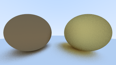
With a sampled sphere of radius 0.5
With a sampled sphere of radius 0.2
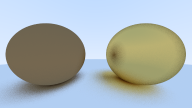
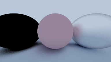
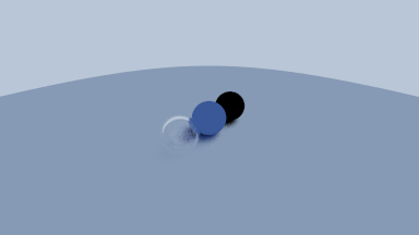
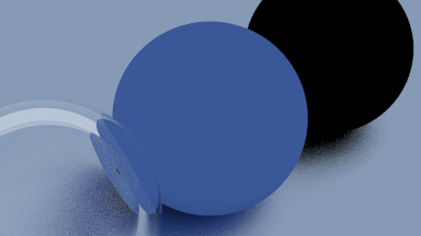
Diffuse, metallic, and fuzzy
Now we’ll see the effects of having the 3 materials in the scene at the same time.
The metallic ball’s albedo is full white, so it doesn’t absorb/attenuate; the ball reflects the exact colors.
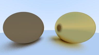
The metallic ball’s albedo is 0.9, 0.9, 0.9, so it attenuates the reflection a little, giving the ball itself some definition.
The metallic ball’s albedo is 0.2, 0.2, 0.2.

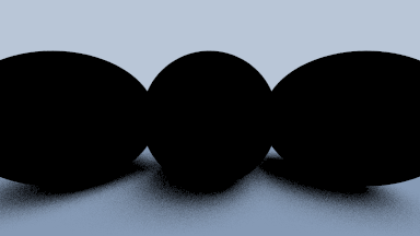
The metallic ball’s albedo is full black. The fuzzy ball’s albedo is full white.
All albedos are black.
Dielectrics and refraction
Dielectrics split a ray into a reflected ray and a refracted ray (the reflected ray is for tinting the surface with the color of nearby surfaces; the refracted ray is for sampling what’s behind the dielectric surface and make it visible through it).
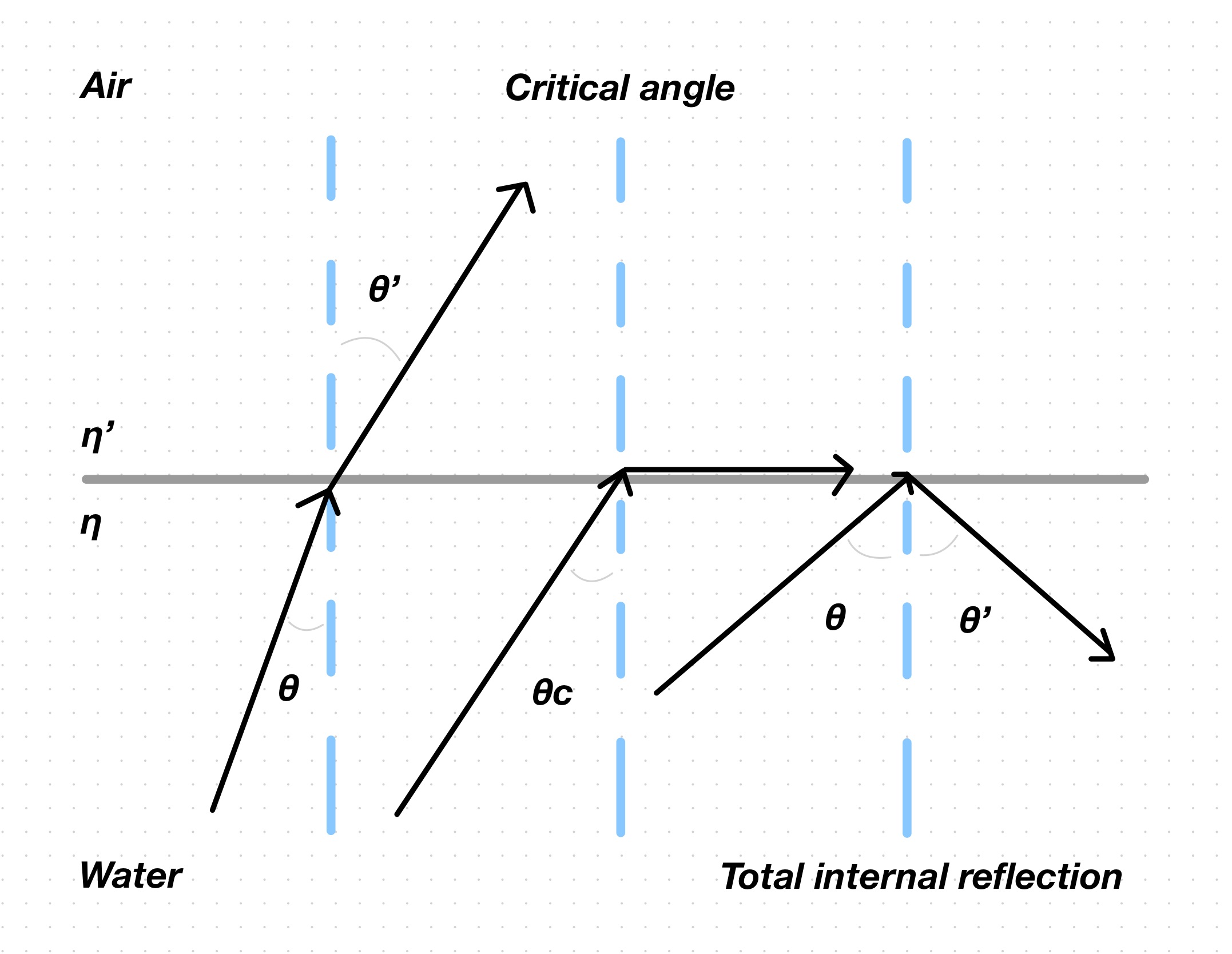
There is a relation between the angle of incidence and the angle of refraction and is ruled by the refractive indices of the media: a ray gets refracted when it transitions from one medium to another; each of these media have its own characteristic refractive index.
\(\eta \sin\theta= \eta' \sin\theta'\) (Snell’s law)
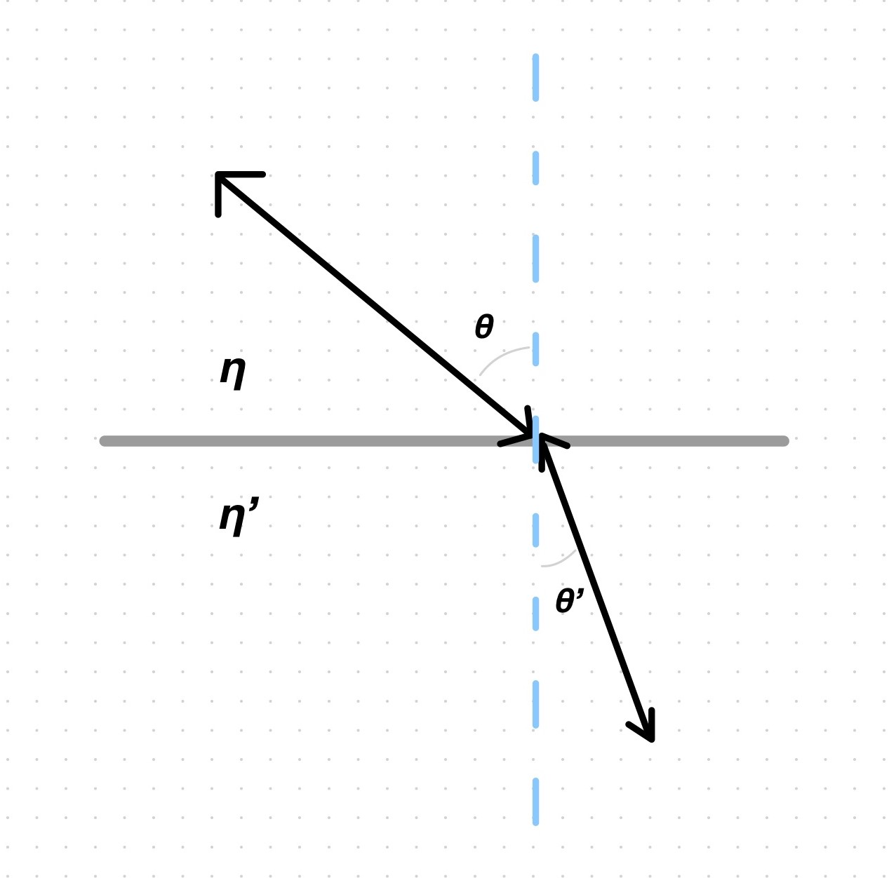
The refractive indices and the angle of incidence are known, so the angle of refraction can be found by solving for it: \[\sin\theta'=\frac{\eta}{\eta'}\sin\theta\]
In ray tracing, we usually don’t know the angles, but we do know the incident ray’s vector \(v\). If \(v\) is normalized:
\(1=\sqrt{1\cos\theta^2+1\sin\theta^2}\) (Pythagorean theorem)
Since \(v\) and \(N\) are normalized: \[\cos\theta=v \cdot N\]
So: \[\begin{aligned} 1 &= \sqrt{(v \cdot N)^2+1\sin\theta^2} \\ 1 &= (v \cdot N)^2+1\sin\theta^2 \\ \sin\theta &= \sqrt{1-(v \cdot N)^2} \end{aligned}\]
Substituting: \[\sin\theta'=\frac{\eta}{\eta'}\sqrt{1-(v \cdot N)^2}\]
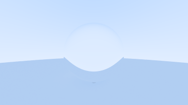
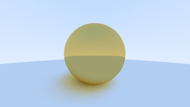
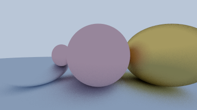
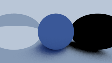
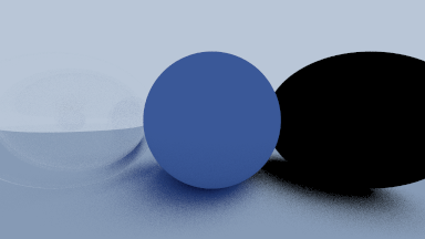
Only refracting
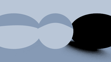
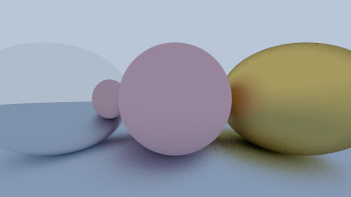
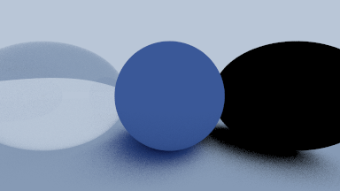
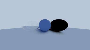
Refracting and reflecting
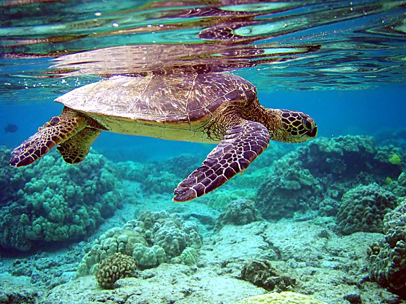
Notice how reflecting gives the ball a sense of grounding. A ball of glass that only refracts is not physically correct anyway. In reality, when a ray moves to a medium with lower refractive index (like from water to air or from the interior of the glass ball to air), there is a threshold or critical angle of incidence past which rays will be reflected at the boundary rather than refracted into the new medium.
Source: Wikimedia Commons
Look at Snell’s law when \(\eta>\eta'\): \[\sin\theta'=\frac{\eta}{\eta'}\sin\theta=\frac{1.5}{1.0}\sin\theta\]
\(\sin\theta'\) has a range of \([-1, 1]\), so the left side of the equation has a maximum value of \(1\). The right side, on the other hand, can exceed \(1\) when \(\theta\) goes past certain angle, because of the \(\frac{\eta}{\eta'}\ge1\) fraction (for example, when \(\sin\theta=1\), the right side will be \(1.5\)). The equality doesn’t always hold. When it doesn’t hold, the boundary turns into a mirror, reflecting the rays back into the 1st medium. In code, we reflect instead of refract when the right side of the equation is larger than \(1\).
Positionable camera
\(2h\) is the height of the viewport. The width of the viewport is obtained from the height by multiplying it by the aspect ratio.
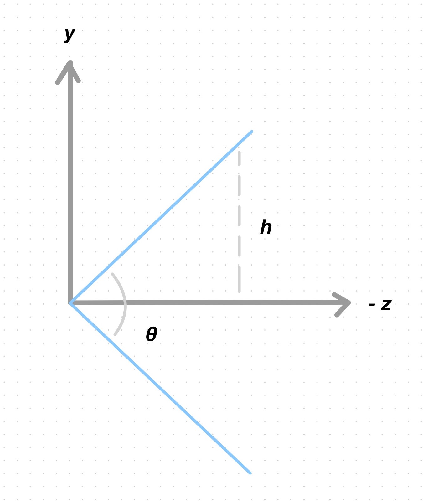
Focal length has an inverse relation to the angle of view and the magnification of the image:
- As focal length gets longer, the angle of view becomes narrower and the scene appears
  magnified.
- As focal length gets shorter, the angle of view becomes wider and the scene is magnified
  less.
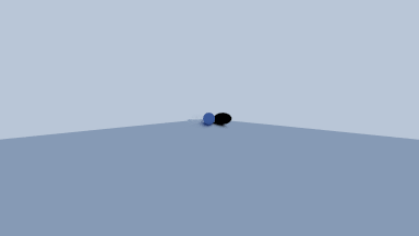
Vertical FOV of \(45°\)

Vertical FOV of \(90°\)
Vertical FOV of \(135°\)
Vertical FOV of \(170°\)
Vertical FOV of \(180°\)

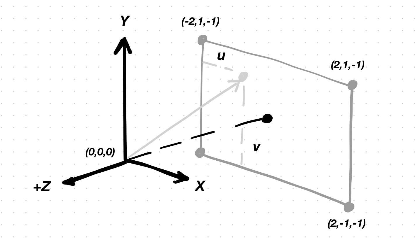
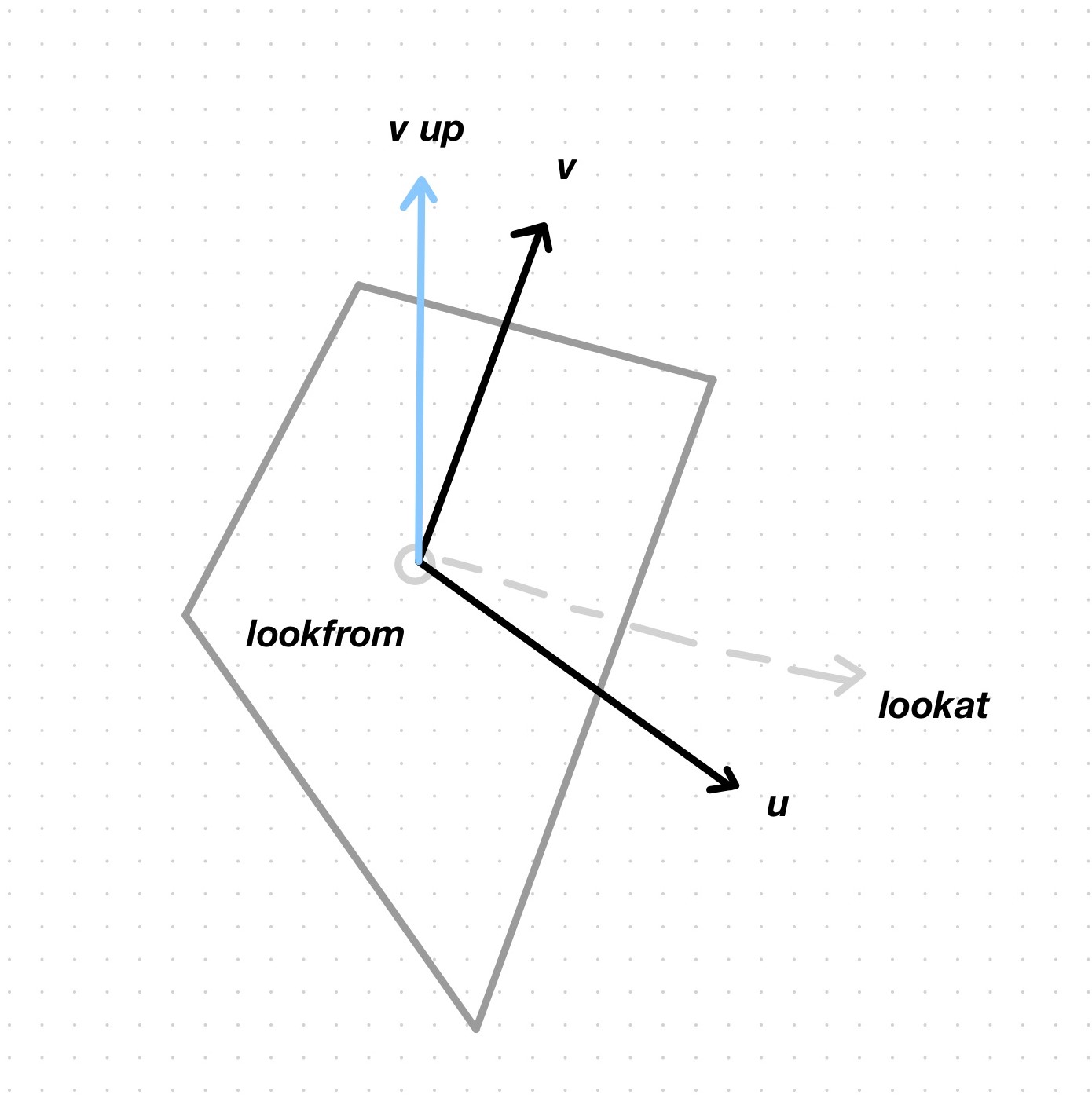
The orientation of the camera can be expressed with an orthonormal basis \((u, v, w)\), where
\(w\) is \(−(lookat−lookfrom)\);
\(u\) is orthogonal to the plane formed by \(w\) and \(v_{up}\) (view up). \(v_{up}\) can be any vector, but \((0, 1, 0)\) is typically used. \(u\) is \(v_{up} \times w\); the cross product produces a vector that is orthogonal to the plane of the other 2. Note that these 2 input vectors don’t need to be ortoghonal to each other;
\(v\) is \(w \times u\).
Now, focus and depth of field. In virtual cameras, everything is in focus. If you want to simulate a physical camera, though, you need to simulate blur. There is a plane in the scene that the camera will capture in perfect focus. The rest of the planes will be blurred. The distance from the camera to this camera focus plane is the focus distance (not to be confused with the focal length).
Blur is achieved in a way similar to antialiasing, i.e. by jittering the ray direction vector. For antialiasing, you randomize the destination point of the ray. For blur, you randomize the source and point of the ray.
